TrackMaster

La versione italiana dello stesso documento è disponibile in docs -> READMEita.md

1. Introduction

Project Purpose

The goal of this knowledge base system is to calculate the necessary values for audio mixing. This process involves playing back the recordings of individual instruments—usually recorded on separate tracks—simultaneously into a single track called master. Consequently, these individual tracks must be modified in order to do so. Furthermore, since these tracks often have generic names like track1, track2, etc... , a subsequent task is to classify and rename each track based on the instrument recorded and the equipment used.

Requirements and Usage

The chosen programming language is Python. The following libraries had been used:

• librosa for analyzing audio track features.
• numpy for array management and numerical operations.
• imbalanced-learn o imblearn specifically for oversampling techniques.
• matplotlib for data visualization and plotting.
• kneed to identify the "elbow" of a curve.
• pandas for dataset manipulation.
• network for managing complex graphs.
• pgmpy for using probabilistic models.
• pydub a wrapper for the ffmpeg audio encoder, used for reading, modifying, and exporting audio files and features.
• seaborn a higher-level specialization of matplotlib.
• scikit-learn for machine learning tasks.

Audio Processing Fundamentals

Mixing is a process that is both creative and highly technical. It consists of combining individual instrument tracks into a single master track. Those are appropriately modified for an optimal sonic result. This project focuses on the following stages of the mix chain:

• Gain the volume at which the track is played. For stereo tracks left and right gain differentiation allows to create a specific stereo image.
• Equalization the gain applied to each frequency of the sound spectrum for every track.
• Compression involves various parameters, including:
  • Threshold the volume level that triggers the compressor.
  • Attack and Release determine how quickly the compressor starts working and how long it continues to operate.
  • Ratio determines the amount of volume reduction. The considered audio equipment is:
• Dynamic Microphones provide good capture of a sound source's dynamics but lose some articulation. Generally preferred for close-miking instruments.
• Condenser Microphones offer excellent sound capture in terms of dynamics, articulation, and frequency response, but tend to easily capture ambient noise or bleed from nearby instruments.
• DI converts an unbalanced audio signal to balanced so that a sound source (e.g., a guitar with a jack) can be recorded with minimal electrical noise.
• Digital used to inform that the track was processed digitally.

2. Considerazioni sul dataset

In order to prepare the dataset, the mixing and mastering of approximately 250 tracks from Telefunken's Live From the Lab was performed using Reaper. This resulted in a dataset where each row contains the equalization, compression, and gain parameters of the original tracks, along with the differences between these features and those of the mixed tracks.
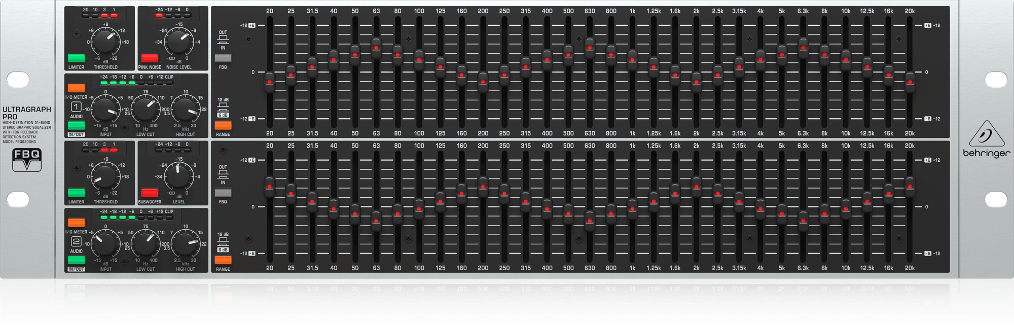
These differences are the values to be predicted, alongside the instrument and equipment. Initially, the project relied on librosa functions to extract features like MFCC coefficients, zero-crossing rate, and spectral centroid. However, these provided an "audio fingerprint" that was not very useful for physical audio modification. Consequently, the focus shifted to features physically used in mixing. Referencing a 31-band graphic equalizer, the system extracts the energy of each frequency in the audible spectrum, the average energy (RMS), peak energy, compression ratio, and left/right channel gain. Compressor attack and release were excluded from the input features as they are default values not calculable from the audio track alone. Including them could have compromised model performance; they appear only as target values. Energy and gain are expressed in dBFS (Decibels relative to Full Scale), a base-10 logarithmic scale ranging from 0dB (maximum) to -144dB. Stereo/mono information was removed to furtherly simplify the models, as it can be retrieved via pyDub or inferred from L/R gain. Missing information regarding instruments, equipment, and genre was manually added. Adding artist and album info could have been useful in case of a bigger dataset. In fact, it's often possible to recognize one from the way their music sounds. The set contains instrument-equipment-genre triples as shown in the following picture
A correlation matrix was produced to understand relationships between numerical components.
The presence of single entries posed the following challenges:

• Overfitting Data is insufficient to generalize patterns for a class especially if trained on a single instance.
• Splitting (Training/Validation/Test) It is impossible to split a single example per class across sets. To mitigate this, a specific test set was created using tracks from the same recording session as the training set, or entirely new tracks with already seen instrument/equipment/genre combinations. It was clear that this solution means corrupting the results.

To further improve quality the genre column was removed. Some instruments were renamed to their macro-category (e.g., mpc and moog were renamed to bassSynth). This solution allowed to significantly reduce the number of single entries. In order to furtherly even the number of class entries some class specialization had been introduced (e.g., floorTom and tom were specified instead of tom only). Being not allowed to modify the resulting master track (being a single entry in a new dataset) mastered tracks were removed from the datasets as they could have been misinterpreted as ambience tracks.
The pre-made testSet was completely abandoned having obtained a more even dataset. The train_test_split function with test_size = 0.11 has been used. Moreover a complete review of the numerical values had been performed on the dataset.

3. Unsupervised Learning

The high number of parameters suggested the use of PCA (Principal Component Analysis) to reduce the number of components, making training more efficient and reducing data related noise. The number of components was calculated to capture 99% of the variance.
Additionally, Clustering was applied to mitigate overfitting. Agglomerative Hierarchical Clustering was the first approach, using Euclidean distance and Ward linkage in order to minimize cluster differences when clustered. Determining the best cluster number (k or height where the dendrogram is to be cut) was a hard task. So different values for k were tested, starting at 54 represetning the number of unique instrument-equipment pairs and halving down to 2.
Cluster entries get unbalanced while reducing k value. This could lead to biased metric results. Consequently, k-Means clustering was also performed. The optimal number of clusters was determined using the elbow method.

4. Metrics

The research aims to find models that return the best metric results. In particular, the following were used for the Classification task:

• accuracy
• precision
• recall
• f1
• log-loss

As for the Regression task:

• r2 score

RMSE hadn't been considered being:

• redundant, being r2 already there;
• unnormalized relative to total variance;
• insignificant, as the dataset includes heterogeneous units such as dB and milliseconds.

5. Classification

The objective is to rename audio tracks.

5.1 Supervisioned Learning

5.1.1 Oversampling

Initially, the adasyn technique was chosen to generate more samples for minority instances. However, it was ultimately discarded because the dataset did not meet the requirement for the number of neighbors to be less than or equal to the number of available samples. Consequently, smotewas selected instead, as it generates samples uniformly across all minority class instances. Nevertheless, since the values identifying each class are very close to one another, this solution does not provide substantial improvements, as documented below.

5.1.2 Decision trees and Kfold

The primary objective of their use is to prevent overfitting and provide a more robust estimate of model performance compared to a single training/test split. To achieve this, StratifiedKFold was employed, as the returned folds preserve the percentage of samples for each class in the dataset. The number of splits used was set to the minimum possible due to the presence of single-entry classes.
After performing label encoding to evaluate predictions for both "instrument" and "equipment," the following models were trained and evaluated. Hyperparameter tuning was conducted via GridSearchCV, utilizing the same StratifiedKFold and optimizing based on the f1_weighted score for each model:

• decision tree, using DecisionTreeClassifier;
• random forest, using RandomForestClassifier. It resulted to be very heavy on hardware resources;
• logistic regression, using LogisticRegression;

5.1.3 Case-Based Reasoning

Given a new target, CBR searches the training set for the cases most similar to the current one. Similarity is measured using th eKNeighborsClassifier (k-NN) after performing label encoding and conducting a hyperparameter tuning for the k-NN itself, utilizing the same StratifiedKFold previously obtained. Subsequently, the number of neighbors that optimizes the f1_weighted score is determined. The solution associated with the most similar past case is then reused to address the new problem.

5.2 Probabilistic Learning

5.2.1 Naive Bayes

Calculate the probability that an instance belongs to a specific class given its features. The goal is to find the class that maximizes the posterior probability P(C|X). The classifier is defined as "naive" because it assumes independence between features, which allows the conditional probability to be written as a product. To achieve this, a Label Encoder was used, followed by GaussianNB, which is specifically designed for continuous independent variables.

5.2.2 Bayesian Network

A DiscreteBayesianNetwork is a type of probabilistic graphical model that represents a set of variables (nodes) and their dependency relationships (edges) through a directed acyclic graph (DAG). Each node is associated with a Conditional Probability Table (CPT), which defines the probability of each state of the node conditioned on the states of its parents. To make the numerical values compatible with the model, they were discretized. The model's edges were identified using the HillClimbSearch algorithm, utilizing the k2scoring function, which is specifically designed to evaluate Bayesian networks based on discrete data. Before selecting K2, other scoring functions were tested:

• BIC (Bayesian Information Criterion), evaluates the network structure using a log-likelihood term combined with a penalty for complexity and overfitting, which resulted in the removal of certain nodes;
• AIC (Akaike Information Criterion), similar to BIC, but the penalty term does not account for the sample size.

k2 was used on all sets where PCA wasn't performed; AIC was otherwise used.

6. Regression

The aim is to predict continuous-value mixing parameters for audio track processing and sound modification.

6.1 Supervised Learning

6.1.1 Linear Regression

Using LinearRegression. It is a statistical method for modeling the relationship between one or more independent variables (X) and a dependent variable (Y). Specifically, the model fits a linear model with coefficients w = (w1, ... , wp) to minimize the residual sum of squares between the observed targets in the dataset and the targets predicted by the linear approximation.

6.1.2 Decision trees

• decision tree using DecisionTreeRegressor
• random forest using RandomForestRegressor. In both regression trees, hyperparameters were obtained performing GridSearchCV, using KFold and optimizing the r2 score.

6.1.3 CBR

Similarity was obtained using NearestNeighbors, optimizing the r2 score.

6.2 Probabilistic Learning

6.2.1 Bayesian Regression

Using BayesianRidge. Hyperparameters were obtained performing GridSearchCV, optimizing the r2 score.

6.2.2 Bayesian Network

Using LinearGaussianBayesianNetwork after performing a HillClimbSearch optimizing the AICgauss scoring.

7. Conclusions

7.1 Results

7.1.1 Classification

Based on the initial results, it was deemed necessary to conduct tests covering as many set combinations as possible, as different preparations of the same sets improve performance and metrics for one model over another.To optimize processing time, it was observed that the sets processed with hierarchical clustering (k = 54 and k = 27) yielded the best metrics; consequently, other values of $k$ were not considered for sets involving only scaling and PCA. Generally speaking, the metric values are poor; therefore, when selecting the best model (highlighted in fuchsia in the figure), greater weight was given to Log Loss and F1 score, respectively. It was not possible to measure metrics for sets with oversampling in any instance, as the number of neighbors consistently exceeded the number of examples—a result of single-instance classes within the sets. The models highlighted in green represent the best results for each specific model type. Regarding the K-Fold cross-validation, two models could technically have been considered "the best," but the one with the lower Log Loss was ultimately selected. The most inefficient model was the Bayesian Network, both in terms of required resources and the results achieved relative to processing time (often exceeding one hour). For this reason, it was omitted from subsequent tests.

7.1.2 Regression

Regarding the impossibility of oversampling mentioned previously, this technique was not considered for this task as it would have introduced noise into the dataset.Compared to the classification task, the metrics are significantly better, with an R2 of zero for the CBR (Case-Based Reasoning). Although this was the best numerical result, the Linear Regression model—trained on a set processed solely with hierarchical clustering (k = 54) — was deemed the superior model. It cannot be ruled out that, in this specific case, the CBR possesses poor generalization capabilities. Furthermore, for the same reasons described above, not all metric fields for the Bayesian Network have been completed.

7.2 Final thoughts

Based on the results obtained, it is possible that the classification task is inherently complex and further complicated by the size of the dataset. Indeed, the modifications made throughout the project did not lead to substantial improvements in metric values. Conversely, the results for the regression task proved to be satisfactory.
Regarding potential future developments, it could be interesting to employ a deep learning model that utilizes the audio spectrogram—represented as an image—as a feature. This approach might yield overall better metric values, given that a track's spectrogram represents everything occurring sonically at every single moment. However, it will be necessary to enrich the dataset with more entries to reduce overfitting and improve the models' ability to generalize.